amibroker

HomeKnowledge Base

Closing trades in delisted symbols

When we perform historical tests on databases that contain delisted symbols – we may encounter a situation, where there are open positions in those tickers remaining till the very end of the backtest, distorting the results (as these open positions will reduce remaining maximum open positions limit for the other symbols).

Here is an easy technique which allows to force closing positions in those symbols on the very last bar traded for given symbol. The code below just adds an additional Sell signal on the last available bar in the database for this symbol:

bi BarIndex();
exitLastBar bi == LastValuebi );
Sell /*your regular sell rules*/ OR exitLastBar

If we are using 1-bar trade delays in our backtesting settings, then the exit signal would need to be triggered one bar in advance (so the delayed signal could still be traded on the last bar) and the code would look like this:

SetTradeDelays(1,1,1,1);
bi BarIndex();
exitLastBar bi == LastValuebi );
Sell /*your regular sell rules*/ OR exitLastBar

There is also a dedicated field in Symbol->Information window which allows to store the delisting date directly in the database. AmiBroker allows to read that field from AFL code using GetFnData() function. If we have this field populated for delisted symbols for our symbols, then the code forcing exits on delisting date would be:

exitLastBar datetime() >= GetFnData("DelistingDate");
Sell /*your regular sell rules*/ OR exitLastBar

What is important, this approach would work also, when Pad and Align to reference symbol feature is used in Analysis window settings.

In order to populate Delisting Date field in the database, we can enter the dates manually through Symbol->Information window or use ASCII importer to import the information from the input text files. More details about ASCII importing can be found at:
http://www.amibroker.com/guide/d_ascii.html

How to identify signal that triggered entry/exit if multiple signals are used

When designing a trading system we often need to quickly identify which of the rules used in the code triggered the particular Buy or Sell signal. Here are some techniques that may be useful in such identification.

For the purpose of this demonstration let us use a sample formula, where the Buy signal may be triggered by one of three independent rules:

Buy1 CrossMACD(), Signal() );
Buy2 CrossCloseMA(Close50) );
Buy3 CrossRSI(), 30 );
//
Buy buy1 OR Buy2 OR Buy3

To determine which of those three rules generates the entry signal, we can either visualize signals in the chart or use Exploration feature of the Analysis window.

In case a custom chart is used, we can do the following:

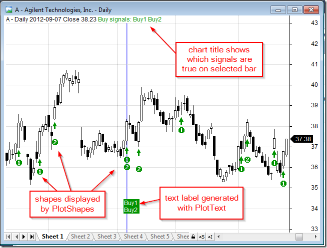
  1. display the signal in custom chart title
  2. use PlotShapes function to indicate certain buy rule
  3. use PlotText to add pre-defined text labels.

The formula below shows sample implementations of these three techniques. This is actually one of many ways that can be used for coding such custom output:

Buy1 CrossMACD(), Signal() );
Buy2 CrossCloseMA(Close,50) );
Buy3 CrossRSI(), 30 );
//
Buy buy1 OR Buy2 OR Buy3;
//
// Standard price plot
PlotClose"Close"colorBlackstyleCandle);
//
// Custom title definition
BuyReason EncodeColor(colorGreen ) + WriteIf(Buy,"Buy signals: ","")
           + 
WriteIf(buy1"Buy1 """) +WriteIf(buy2"Buy2""")
           + 
WriteIf(buy3"Buy3""");
Title StrFormat"{{NAME}} - {{INTERVAL}} {{DATE}} Close %g ",Close ) +BuyReason;
//
// Plotshapes function calls
PlotShapes(Buy*shapeUpArrowcolorGreen0Low);
PlotShapes(Buy1*shapedigit1colorGreen0Low,-30);
PlotShapes(Buy2*shapedigit2colorGreen0Low,-45);
PlotShapes(Buy3*shapedigit3colorGreen0Low,-60);
//
//
// Custom text labels displayed with PlotText
if( SelectedValue(Buy) )
{
   
SelectedValueBarIndex() );
   
maxy Status("axismaxy");
   
miny Status("axisminy");
   
0.15 * (maxy miny) + miny;
   
text WriteIf(buy1], "\nBuy1 """)
          +  
WriteIf(buy2], "\nBuy2 """)
          +  
WriteIf(buy3], "\nBuy3 """);
   
PlotTexttexti,  ycolorWhitecolorGreen );

The chart below shows how to use signal visualization technique implemented in the formula.

Chart Example 1

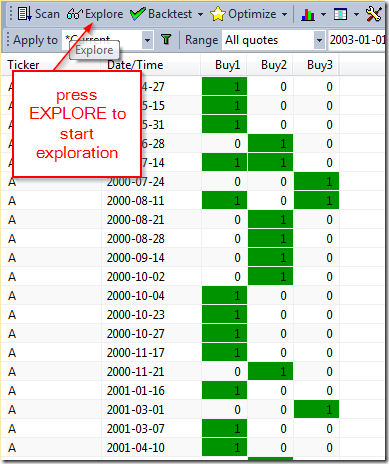
The other method is to use the Exploration feature of Analysis window that allows to generate tabular output, where we can display the values of selected variables. The detailed tutorial explaining this feature is available at:
http://www.amibroker.com/guide/h_exploration.html

For the discussed purpose of tracking the signals that triggered entry or exit, we can add the following code to our trading system to show the values of each Buy1, Buy2, Buy3 variables:

Filter Buy;
AddColumnBuy1"Buy1"1colorDefaultIIfBuy1colorGreencolorDefault ) );
AddColumnBuy2"Buy2"1colorDefaultIIfBuy2colorGreencolorDefault ) );
AddColumnBuy3"Buy3"1colorDefaultIIfBuy3colorGreencolorDefault ) )

Exploration Signal tracking

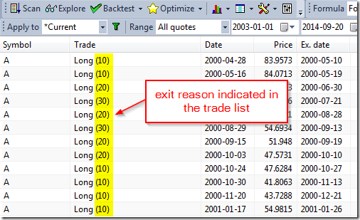
With regard to exit signals they can be visualized in a similar way as shown above, but there is also an additional functionality in the backtester, which allows to indicate the exit condition directly in the trade list. This can be done by assigning values higher than 1 (but not more than 127) to Sell variable.

Sell1 CrossSignal(), MACD() );
sell2 CrossMA(Close50), Close );
Sell Sell1 10 Sell2 20

The above expression will result in assigning value of 10 to Sell variable for the bars where Sell1 is true, 20 for the bars where Sell2 is true and 30 for the bars where both conditions are true.

These values will be indicated in the trade list:

Backtest exit signal tracking

It is worth to mention that values 1 to 9 are reserved for built-in stops and used internally by the backtester, and have special meaning:

  1. normal exit
  2. maximum loss stop
  3. profit target stop
  4. trailing stop
  5. n-bar stop
  6. ruin stop (losing 99.96% of entry value)
  7. reserved
  8. reserved
  9. reserved

Note also that you must not assign value greater than 127 to Sell or Cover variable. If you assign bigger value it will be truncated.

This is further discussed here: http://www.amibroker.com/guide/afl/equity.html

Broad market timing in system formulas

Some trading systems may benefit from attempt to time the broad market. A market-wide valuation, such as moving average, sentiment or some other mechanism may be used to tell if we should be in the market or not.

Flexibility of AFL language allows to create rules or indicators, which are based on more than just one symbol. This enables us to introduce additional filters based on wide-market index performance.

For the purpose of reading quotes of another symbol one can use Foreign or SetForeign functions.

The following formula shows how to generate entry signals in individual stocks when S&P500 index is above its 200-period moving average and exit signals when S&P500 is equal or below 200-period average (^GSPC is a ticker for Yahoo Finance data for S&P500)

//
// read S&P 500 values from ^GSPC ticker
//
sp500 Foreign"^GSPC""C" );
//
// market-wide filter should be in "state" form
// (so it is True all the time when market is up)
//
marketup sp500 MAsp500200 );
marketdown NOT marketup;
//
// sample trading rules (MACD crossovers)
//
BuySignal CrossMACD(), Signal() );
SellSignal CrossSignal(), MACD() );
//
// combine per-symbo signals with broad-market timing
//
Buy BuySignal AND marketup// enter trade only when buy signal AND market is in up trend
Sell SellSignal OR marketdown// exit position if sell signal OR market turns dow

A more complex broad-market timing that requires not only closing price of market index can be implemented using SetForeign function. SetForeign replaces all OHLCV data series with that of the “other” security and allows to calculate all kind of indicators that would normally use current security. Broad market timing does not need to be just “all-in” or “all-out” switch. For example one can switch the trading method depending on whenever broad market is trending or sideways.

//
// Switch to S&P symbol to calculate broad-market timing
//
SetForeign"^GSPC" );
//
// now we can calculate any indicator based on SP500
//
MarketIsTrending ADX40 ) > 20// ADX (40 days) from SP500
//
// now go back to original data (current symbol)
//
RestorePriceArrays();
//
// you can have different rules that are switched
// depending on what broad market is doing
//
TrendingBuy CrossCMAC30 ) );
TrendingSell CrossMAC30 ), );
//
SidewaysBuy CrossMACD(), Signal() );
SidewaysSell CrossSignal(), MACD() );
//
// switch methods using broad-market timing
//
Buy IIfMarketIsTrendingTrendingBuySidewaysBuy );
Sell IIfMarketIsTrendingTrendingSellSidewaysSell )

In this simple example we assume that market timing signals change very infrequently so they change much less often than Trending/Sideways Buy/Sell signals are generated. If that is not the case the switching logic would need to be more complex to decide what to do when we are in the “trending” trade and market switches to sideways mode. In such situation, the code above uses SidewaysSell signal to sell the position, which may or may not be what you are after.

Another example is changing position sizing depending on broad market conditions. We can choose to be fully invested when broead market is up and only 30% invested in down market.

//
// Switch to S&P symbol to calculate broad-market timing
//
SetForeign"^GSPC" );
//
// now we can calculate any indicator based on
// SP500
//
MarketIsUp MAC200 ); // here C represents closing price of SP500
//
// now go back to origiginal data (current symbol)
//
RestorePriceArrays();
//
// normal rules (in this example they do not chang)
//
Buy CrossMACD(), Signal() );
Sell CrossSignal(), MACD() );
//
// no more than 10 positions open at a time
//
SetOption("MaxOpenPositions"10 );
//
// change position sizing depending on broad market conditions
// in this example we will allocate:
// 10% per position
// if broad market is up (so we can be allocated upto 100% of funds)
// 3% per position
// if broad market is down (so we can be allocated upto 30% of funds)
//
SetPositionSizeIIfMarketIsUp10), spsPercentOfEquity )

How to print result list from Analysis window

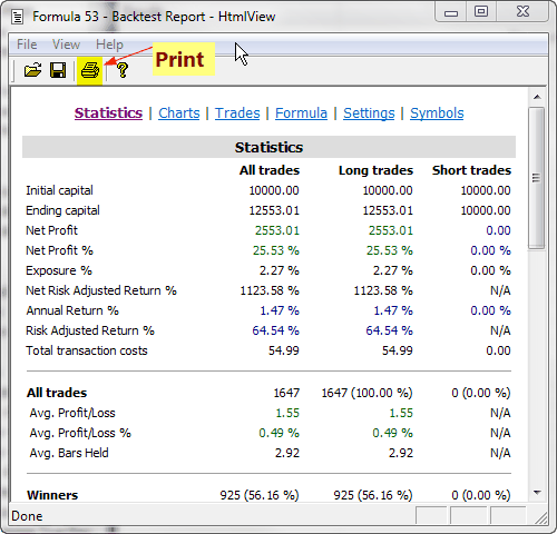
As far as backtest results are considered, they can be printed directly from Report Viewer.

Report printing

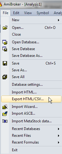
But sometimes we may want to print just the result list of scan, exploration or optimization. In order to print out the results list from Analysis window it is necessary to store the results list into a file first. This can be achieved by using File->Export HTML/CSV option from the main menu of the program (Export option is available when Analysis window is open):

Export

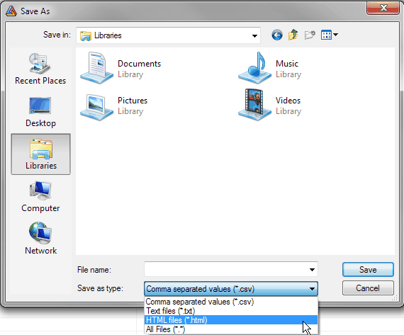
I recommend saving in HTML format as only then color output will be preserved.

Export as HTML

Once the result list is saved to a HTML file, you can double click on the file to open it with your default web browser. From web browser you can choose Print option.

If you prefer to modify the file prior to printing you can also save the result list in CSV format that can be open with Excel or any other application of your choice.

An alternative solution is to use system clipboard and to copy the results (using Ctrl+C keyboard shortcut or Copy option from the context menu available under right-mouse button), paste to the application like MS Excel for example and printing the results there.

Too small / unreadable Profit Table in the backtest report

Some of users may observe that their Profit table is too small, so the numbers get truncated or the text is too small.

First let me tell you that profit table in the backtest report is not really a table, but a bitmap image with fixed dimensions. Profit table, like any other user-definable report chart, is created by running an AFL formula present in the “Report charts” subfolder. The chart is rendered into bitmap image that gets later embedded in the backtest report.

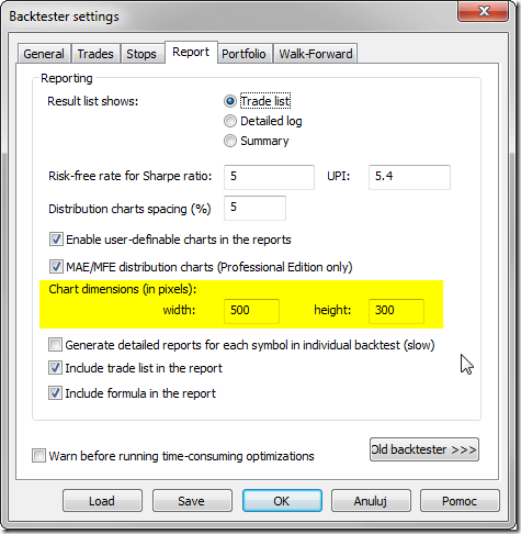
The size of backtest report images depends on Analysis window settings. In order to increase the size of generated images, it is necessary to go to Analysis -> Settings, Report tab and increase the picture dimensions:

reportchartdim

Once you change it, newly generated reports will use enlarged image dimensions. Adjusted settings will affect new backtests only, but not the old reports that have already been generated.

Tip: You can create your own report charts by placing your own AFL formula in the “Report charts” subfolder.

Why do backtest results change?

From time to time we receive questions about why you can get different results back-testing the same code.

There are many reasons for differences in backtest results:

  1. Different data

    For example if past history is updated/changed due to splits for example or backfill or external data update.

  2. Different settings / parameters

    May happen if your formula uses Param() functions that output values that may be changed from the Parameter window.

    Note that Parameters in Analysis window use shared ChartID=0, which means that if two formulas use same parameter names they would share parameter values as well.

  3. Different formula

    Sometimes even slight change to the formula causes big change in the results, for example if your formula uses #include and included code has changed

  4. The formula that self-references its previously generated results.

    Such code produces some data that is later used to produce next run output (for example your code produces composites that are later used – if those composites change – the input data change so the results change, or if your formula uses previous backtest equity or if your formula uses STATIC variables without deleting/clearing them at the beginning)

  5. The formula uses random number generator

    This occurs when your formula directly or indirectly calls any function that produces random numbers such as Random or mtRandom

  6. The formula reads external files/data that might have changed

    This occurs when your formula directly or indirectly calls any functions that read external files or data that have changed between backtests. It can be as trivial as using current time in your formula.

  7. The formula sets global (per-backtest) settings to non-constant value – for example sets global option differently for each symbol.

    This one is subtle and can be easily overlooked by non-experienced users. One has to understand that global (per-backtest) settings are applied to entire portfolio. If one changes those settings on per-symbol basis, then “last write” counts, and it means that result of your backtest will depend on which execution thread ended last. In Windows OS, it is generally unpredicatable which thread ends first because of so many factors that affect execution time. So your backtest may use different settings in different runs as a result of this. Bottom line: never change global settings in your formula to non-constant value.

Using Zig-Zag in trading systems

Zig-zag indicator, as well as other functions using it (Peak/Trough, PeakBars, Troughbars), inherently look into the future. As such they should not be used in trading system formulas without taking precautions. The only way to fix the ‘problem’ is to delay the signal as long as it takes for zig/zag to stabilise last ‘leg’. The delay is variable and depends how much time it takes for defined percentage change to occur in the price series since last peak/trough.

Ready-to-use solution is presented in the Traders’ Tips section of the AmiBroker members area:
http://www.amibroker.com/members/traders/11-2003.html

(NOTE: access to members’ area is limited to licensed users only, if you forgot your password use reminder at http://www.amibroker.com/login.html)

Points-only backtest

Some users coming from Metastock ask for “points-only” test.

One needs to know that AmiBroker features way more sophisticated futures mode than MS ever had: http://www.amibroker.com/guide/h_futbacktest.html
It provides full support for futures trading, handling margin deposit, point value, etc.

“Points-only” test is kind of the simplest possible case, but if you want to do just that, it can be implemented using these two lines:

SetOption("FuturesMode"True );
SetPostionSize1spsShares ); // trade just 1 contrac

That is all what you need to add to your formula to get point-only test.

Historical portfolio backtest metrics

Recently on the AmiBroker mailing list some users expressed wish to have access to some of portfolio backtest metrics available in “historical” form (i.e. as date series, as opposed to scalars), so they can be plotted as an indicator.

Implementing such functionality is actually easy with existing tools and does not require any OLE scripts. Everything you need is small custom-backtester procedure that just reads built-in stats every bar and puts them into composite ticker.
In the accompanying indicator code all you need to do is simply use Foreign() function to access the historical metrics data generated during backtest.

The code below shows the BACKTEST formula with custom backtester part:

// Replace lines below with YOUR TRADING SYSTEM
EnableRotationalTrading();
PositionScore 1/RSI(14);
PositionSize = -25;
SetOption("WorstRankHeld");
SetOption("MaxOpenPositions"); 

////////////////////////////////////////
// BELOW IS ACTUAL CUSTOM BACKTESTER PART
// that can read any built-in metric (in this example UlcerIndex)
// and store it into composite ticker for further
// retrieval as data series

SetOption("UseCustomBacktestProc"True ); 

if( 
Status("action") == actionPortfolio )
{
  
bo GetBacktesterObject();

  
bo.PreProcess(); // Initialize backtester

  // initialize with null
  // you can have as many historical metrics as you want
  // (just duplicate line below for many metrics you want)
  
MyHistStat1 Null;
  
MyHistStat2 Null// add your own 

  
for(bar=0bar BarCountbar++)
  {
   
bo.ProcessTradeSignalsbar );
  
   
// recalculate built-in stats on EACH BAR
   
stats bo.GetPerformanceStats); 
 
   
// the line below reads the metric and stores it as array element
   // you can add many lines for each metric of your choice
   
MyHistStat1bar ] = stats.GetValue("UlcerIndex"); // get ulcer index value calculated this bar
   
MyHistStat2bar ] = stats.GetValue("WinnersPercent"); // add your own

  
}

  
bo.PostProcess(); // Finalize backtester

  // now STORE the historical data series representing the metric of your choice
  // duplicate the line below for as many metrics as you want
  
AddToCompositeMyHistStat1"~~~UI_HISTORICAL""X"atcFlagEnableInPortfolio atcFlagDefaults );

  
// you can add your own as shown below
  
AddToCompositeMyHistStat2"~~~WP_HISTORICAL""X"atcFlagEnableInPortfolio atcFlagDefaults ); 

In the code above, for illustration purposes, we are exporting UlcerIndex and Winners Percent metrics as data series. They are stored in composite tickers for easy retrieval from indicator level.
You can easily extend code to include ANY number of metrics you want.

Now in order to Plot metrics as indicators, use this simple formula:

PlotForeign("~~~UI_HISTORICAL""UlcerIndex Historical"colorRedstyleLine );
PlotForeign("~~~WP_HISTORICAL""Winners Percent"colorBluestyleLine styleOwnScale )

As you can see with one Foreign function call you can read the historical value of any metric generated by the backtester.

NOTE: when running backtest please setup a filter in AA that EXCLUDES composites (group 253) from backtest set.

Getting started with automatic Walk-Forward optimization

Recently released AmiBroker 5.05 BETA features the automatic Walk-Forward Optimization mode.

The automatic Walk forward optimization is a system design and validation technique in which you optimize the parameter values on a past segment of market data (“in-sample”), then test the system forward in time on data following the optimization segment (“out-of-sample”). You evaluate the system based on how well it performs on the test data (“out-of-sample”), not the data it was optimized on.

To use Walk-Forward optimization please follow these steps:

  1. Goto Tools->Automatic Analysis
  2. Click Settings button, then switch to “Walk-Forward tab”
  3. Here you can see Walk forward settings for In-sample optimization, out-of-sample backtest
    “Start” and “End” dates mark initial period begin / end
    This period will be moved forward by “Step” until the “End” reaches the “Last” date.
    The “Start” date can move forward by “step” too, or can be anchored (constant) if “Anchored” check is on.
    If you mark “Use today” then “Last” date entered will be ignored and TODAY (current date) will be used instead

    By default an “EASY MODE” is selected which simplifies the process of setting up WF parameters.
    It assumes that:
    a) Out-of-sample segment immediatelly follows in-sample segment
    b) the length of out-of-sample segment equals to the walk-forward step

    Based on these two assumptions the “EASY” mode takes in-sample END date and sets
    out-of-sample START date to the following day. Then adds in-sample STEP and this becomes out-of-sample END date.
    In-sample and Out-of-sample step values are set to the same values.

    The “EASY” mode guarantees correctness of WF procedure settings.

    In the “ADVANCED” mode, the user has complete control over all values, to the extent that
    they may not constitute valid WF procedure.
    The interface allows to selectivelly disable in-sample and out-of-sample phases using checkboxes at top
    (for special things like runnign sequential backtests without optimization).

    All settings are immediatelly reflected in the PREVIEW list that shows all generated IS/OOS segments and their dates.

    The “Optimization target” field defines the optimization raport COLUMN NAME that
    will be used for sorting results and finding the BEST one. Any built-in column can be used
    (as appears in the optimization output), or you can use any custom metric that you define
    in custom backtester. The default is CAR/MDD, you can however select any other built-in metric from the combo.
    You can also TYPE-IN any custom metric that you have added via custom backtester interface.

  4. Once you defined Walk-Forward settings, please go to Automatic Analysis and
  5. press the dropdown ARROW on the Optimize button and select “Walk Forward Optimization”

This will run sequence of optimizaitons and backtest and the results will be displayed in the “Walk Forward” document that is open in the main application frame.
When optimization is running you can click “MINIMIZE” button on the Progress dialog to minimize it – this allows to see the Walk Forward output during the optimization steps.

IN-SAMPLE and OUT-OF-SAMPLE combined equity

Combined in-sample and out-sample equities are available by
~~~ISEQUITY and ~~~OSEQUITY composite tickers (consecutive periods of IS and OOS are concatenated and scaled to
maintain continuity of equity line – this approach assumes that you generally speaking are compounding profits)
To display IS and OOS equity you may use for example this:

PlotForeign("~~~ISEQUITY","In-Sample Equity"colorRedstyleLine);
PlotForeign("~~~OSEQUITY","Out-Of-Sample Equity"colorGreenstyleLine);
Title "{{NAME}} - {{INTERVAL}} {{DATE}} {{VALUES}}"
« Previous PageNext Page »