amibroker

HomeKnowledge Base

Limits of multithreading

From time to time users approach us asking various questions related to multithreading such as:

  1. Why his/her formula does not run 32 times faster on 16 core / 32 thread computer
  2. Will 16 core processor be twice as fast as 8 core
  3. Why their CPU does not show 100% usage?

The reason of all those questions is lack of understanding of multithreading and laws governing computing in general.

In this article we will try to address some of those misunderstandings and misconceptions. We assume that the reader already read Efficient use of multitreading from AmiBroker’s Users’ guide and is fully aware how work is distributed in many threads in the Analysis window. We also assume that the reader already read Peformance Tunning chapter of AmiBroker’s guide. These two parts of the manual explain fundamental concepts and are essential to understanding of what is written below.

Another fundamental reading is Amdahl’s Law article in the Wikipedia that explains theoretical speedup limit of any multi-threaded program. In short Amdahl’s law says that if 95% of your program runs in multiple threads and only 5% of it is serial (single-threaded), the maximum achievable speedup regardless of how many CPUs and how many cores you have is 20x (20 times).

Let us focus on Analysis window performance (Exploration/Scan/Backtesting/Optimization). Any operation in the Analysis window involves:

  1. preparing data (this involves reading data from the database, data compression to selected interval, filtering, padding, etc)
  2. setting up AFL engine for execution (setting up built-in arrays, stops, parsing of your formula)
  3. execution of your formula (in backtest for example it means first phase of backtest run, done on every symbol)
  4. per-symbol processing the output of your formula (in backtest it is sorting signals by position score)
  5. post-processing (in case of portfolio backtest it is for example portfolio backtest phase that is done once per backtest, NOT for every symbol)

AmiBroker is highly parallel multithreading application, so most of steps are done in multiple threads. Specifically only first and last (1. and 5.) step is serial, the rest (2, 3, 4) is parallel. It is worth noting that steps 1-4 are done on every symbol, while step 5 is only done once for all symbols. In addition to that program spends some time handling the UI (things like updating UI controls like progress bar and reacting to your mouse / keyboard input) which is of course done in single (main) UI thread.
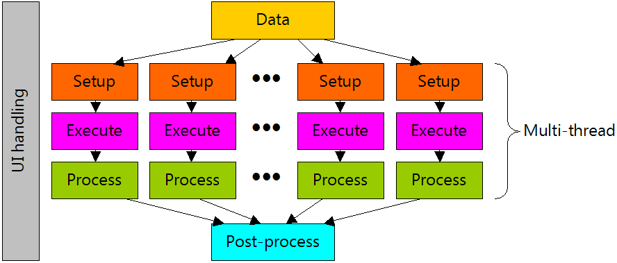
Multitreading 1

There is one exception, a special case: Individual optimization. In individual optimization step 1 is done only once (for one symbol), and all other steps 2-5 (so including last one) are done in multiple threads.
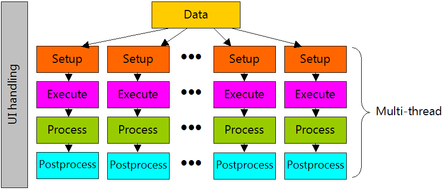
Multitreading 2

Now is where Amdahl’s law kicks in. By adding threads/cores/processors you can only decrease parallel parts (2..4 or 2..5) and ultimately you are limited by the speed of data access. You can’t backtest faster than you can read/prepare the data.

As for data access: the database is shared resource, no matter where it resides. If it resides on hard disk, it is single physical device that does not speed up with increasing number of CPUs. If it resides in RAM, it is still single physical RAM, that has limit on bandwidth and fixed latency regardless how many processors you throw to the mix. Even if it is in L3 (Level 3) cache on the processor, it is still single L3 cache shared by multiple cores. And it is worth nothing, that L3 cache even on most modern processors operate on half the speed of the core, so single core can actually saturate bandwidth of L3 cache if doing nothing but reading or writing large chunks of data from/to it. In many cases this means that processor must wait for memory, unless it is doing complex computations involving only minimum amount of data. These are for example real-world measurement results for triple channel RAM controller on Intel i7 920 CPU (measured using memtest86 program)

Data location  Bandwidth [MB/sec]
L152408
L230722
L324521
RAM11879

Only L1 cache runs at full core speed. As you can see L3 cache has half the bandwidth and RAM has 1/4 of bandwidth of L1 cache. Of course disk speeds (even SSD) are far cry behind 11GB/sec offered by RAM.

In case of portfolio backtest: a final backtest phase (portfolio backtesting) is one per backtest, done once for all symbols, so naturally it is done in single thread (as opposed to first phase that is done on every symbol in parallel).

Now, knowing this all you may wonder how to use all that knowledge in practice.

For example it allows to understand the limits of achievable speed gains for given formula and plan your hardware purchases or find ways to improve run times.

As we learned from the above the only parts that can be speed-ed up by adding more cores are those that are run in parallel (multiple threads). In practice it means – your AFL formula code. What is more the more time is spent in parallel part the better it scales on multiple cores. This means that simple formulas DO NOT scale too well because they are too simple to put enough strain on CPU and are mainly memory (data access) bound. All your simple moving average cross overs are just too simple to keep CPU busy for longer time, especially when there is not too much data to process.

Let us take this trivial formula for example:

period Optimize"period"102102);
Buy CrossCMACperiod ) );
Sell CrossMACperiod ), )

and run Optimize->Individual Optimize on symbol that has 2000 quotes.

Now switch to “Info” tab in the Analysis window and you will see this output (this example comes from 4 core / 8 thread Intel i7), all times are in seconds:

Individual optimize started.
Completed in 0.49 seconds. Number of rows: 500
( Timings: data: 0.11, setup: 0.00, afl: 0.28, job: 2.97, lock: 0.00,
pbt: 0.00, UI thread: 0.11, worker threads: 3.26/3.26 )

So our 500 step optimization on 2000 quotes took less than half of the second. What you see there are some cryptic numbers that you might wonder what they mean. Here is the explanation (for the backtest/optimization)

a) data – time spent accessing/preparing the data
b) setup – time spent preparing AFL engine
c) afl – time spent executing your formula (first phase of backtest)
d) job – post processing (here signals are collected and trading simulation is performed in case of individual optimize)
e) lock – time spent waiting in critical section / lock accessing shared signal table
f) pbt – portfolio backtesting code (not used in individual optimization)
g) UI thread – time spent in UI thread in total (data + pbt + UI handling) – single threaded time
h) worker threads – time spent in worker (parallel) threads (setup+afl+job+lock) – multi-threaded time

Firstly it may look surprising that “worker threads” time is 3.26 which is way longer than entire optimization took (0.49 seconds). But this time is a SUM of times spent in all 8 threads. They ran in parallel. Each was running for (3.26/8 seconds = 0.4075 seconds), and with only one thread running it would take 3.26s. Now you suddenly realize the power of multi-threading!

So now it would seem that our formula run (0.11 + 3.26)/0.49 = 6.8 times faster than on single core.

You may ask why not 8x? We had 8 threads, didn’t we?

First reason is the Amdahl’s law – serial time (0.11sec) is constant and limits our speed up, no matter how many threads you would put on it, but there is something more.

Let us check how much time would it really take if we limited to one thread only. Try running with #pragma statement limiting number of threads:

#pragma maxthreads 1
period Optimize"period"102102);
Buy CrossCMACperiod ) );
Sell CrossMACperiod ), )

Suddenly the result is:

Individual optimize started.
Completed in 1.62 seconds. Number of rows: 500
( Timings: data: 0.07, setup: 0.00, afl: 0.10, job: 1.37, lock: 0.00,
pbt: 0.00, UI thread: 0.07, worker threads: 1.47/1.47 )

What? Entire optimization took just 1.62 seconds when run in single-thread which is just 3.3 times slower than multi-threaded, not 6.8x as we calculated earlier. Why worker thread is 1.47 ? It was 3.26? What happened?

There are couple of reasons for that:
a) Hyper-threading – as soon as you exceed CPU core count and start to rely on hyperthreading (running 2 threads on single core) you find out that hyperthreading does not deliver 2x performance. If your code is NOT doing complicated things like lots of trigonometric functions that put FPU busy or other number crunching, the hyperthreading will not give you 2x performance. On simple tasks it struggles to deliver +30%.
b) Turbo boost – modern CPUs have different settings for single-core turbo boost and multi-core turbo boost. The effect is that CPU can reach raise clock to 4GHz when running single-core only but limit to 3.5GHz when running multi-threaded code. This limits multi-threaded performance and speeds up single-thread apps
c) Concurrent L3 cache / RAM access – when multiple cores run the code accessing L3 cache / RAM they will fight for access slowing them down

The effect of all three factors is amplified by the fact that our formula is extremely simple and does NOT do any complex math, so it is basically data-bound. This is why single-core execution was not as bad as we expected.

But what would happen if we increase the number of bars (keeping formula the same)? Let us try with 12000 bars of data (6 times more data than previously):

8-threads:

Individual optimize started.
Completed in 1.61 seconds. Number of rows: 500
( Timings: data: 0.18, setup: 0.00, afl: 0.81, job: 11.57, lock: 0.00,
pbt: 0.00, UI thread: 0.19, worker threads: 12.38/12.38 )

1-thread:

Individual optimize started.
Completed in 6.90 seconds. Number of rows: 500
( Timings: data: 0.10, setup: 0.00, afl: 0.28, job: 6.48, lock: 0.00,
pbt: 0.00, UI thread: 0.10, worker threads: 6.76/6.76 )

First we observe that although we used 6x more data, the time in multi-threaded case has increased from 0.49 to 1.61 which is only 3.28x. Secondly we see that 8-threaded execution is now 6.90/1.61 = 4.29 times faster than single-threaded.

What happened that multi-threaded performance is now better and it scales better?

Simply – we loaded CPU with more work. That is general rule, the more work you place on the CPU, the more time is spent in parallel section and more gain you get from multi-threading.

So, what would happen if you put CPU to some really heavy-work. It is surprisingly difficult to put i7 CPU into such a hard work that it sits busy doing calculations and not doing too much memory access. You would really need to use functions that do heaps on calculations on very small chunks of data sitting in L1 cache all the time or use some transcendental math functions that require FPU to spend way more than single cycle to derive result. Let us try with combination of raising to power, decimal logarithm and arcus sine.

period Optimize"period"102501);
Buy CrossCMACperiod ) );
Sell CrossMACperiod ), );
// add some math to force i7 CPU to sweat a little bit
for( 0100i++ ) acoslogperiod ) )

Once you to run this you will see AmiBroker saturating your CPU (on my end it uses 99% of CPU) for the first time. The results are:

8 threads:

Individual optimize started.
Completed in 39.39 seconds. Number of rows: 500
( Timings: data: 0.14, setup: 0.00, afl: 302.73, job: 9.14, lock: 0.00,
pbt: 0.00, UI thread: 0.14, worker threads: 311.87/311.87 )

1 thread:

Individual optimize started.
Completed in 251.27 seconds. Number of rows: 500
( Timings: data: 0.12, setup: 0.00, afl: 243.92, job: 6.59, lock: 0.00,
pbt: 0.00, UI thread: 0.12, worker threads: 250.51/250.51 )

Now you can see that 8 threaded execution was (251.27/39.39) 6.38 times faster than single-threaded.

This is almost perfect scaling with hyperthreading – remember hyper-threaded thread is NOT fast as separate-core thread. To prove that we can run same code on 4 threads:

#pragma maxthreads 4
period Optimize"period"102501);
Buy CrossCMACperiod ) );
Sell CrossMACperiod ), );
// add some math to force i7 CPU to sweat a little bit
for( 0100i++ ) acoslogperiod ) )

With four threads we get:

Individual optimize started.
Completed in 64.63 seconds. Number of rows: 500
( Timings: data: 0.13, setup: 0.00, afl: 250.22, job: 6.91, lock: 0.00,
pbt: 0.00, UI thread: 0.13, worker threads: 257.12/257.12 )

So 4-thread performance was 251.27/64.63 = 3.89 faster than single-thread. And look at the “worker threads” time it is very close to single-thread time (250s vs 257s). This proves our point that except the effect of RAM and L3 congestion and slightly slower turbo boost speed, full-core threads scale perfectly as long as your formula puts them into some real work.

Note: in all those tests we did NOT include the impact of disk speed because we run single-symbol individual optimization which runs out of RAM.

Bottom line is: despite marketing hype buying 32 thread CPU does not buy you 32x performance. Real-world performance depends on many factors including formula complexity, whenever it is heavy on math or not, amount of data, RAM speed, on-chip cache sizes, turbo boost clocks differences between single-thread and multi-thread configurations and so on. The devil is in the details and there are no simple answers. I always say: do not assume. Assumptions are not facts. Unless you measure something you don’t know.

Long-only rotational back-test

Rotational trading is a kind of backtest where you trade by switching positions between various symbols based on their relative score instead of traditional buy/sell/short/cover signals.

Since there are no signals used, only PositionScore assigned to given symbol matters.

It is worth noting that in case of rotational test, the Positions field in General tab of the Analysis settings is ignored. It is only used for regular backtests that use actual buy/sell/short/cover signals.

In the rotational mode the trades are driven by values of PositionScore variable alone.

In particular:

  • higher positive score means better candidate for entering long trade
  • lower negative score means better candidate for entering short trade

As you can see the SIGN of PositionScore variable decides whenever it is long or short.

Therefore – if we want to test long-only system in rotational backtesting mode, then we should use only positive values in PositionScore variable. For example – if we are trading a system, which uses 252-bar rate of change for scoring purposes:

SetBacktestModebacktestRotational );
SetOption("MaxOpenPositions",5);
SetOption("WorstRankHeld",5);
SetPositionSize20spsPercentOfEquity );
PositionScore ROCClose252 )

Then, to trade only long positions, we should change PositionScore defintion for example to:

PositionScore 1000 ROCClose252 ); // make sure it is positive by adding big constan

This way our scores will remain positive and that will effectively disable short trades.

More information about the rotational mode of the backtester can be found in the manual: http://www.amibroker.com/guide/afl/enablerotationaltrading.html

Separate ranks for categories that can be used in backtesting

When we want to develop a trading system, which enters only N top-scored symbols from each of the sectors, industries or other sub-groups of symbols ranked separately, we should build appropriate ranks for each of such categories. This can be done with ranking functionalities provided by StaticVarGenerateRanks function.

The formula presented below iterates though the list of symbols included in the test, then calculates the scores used for ranking and writes them into static variables. The static variables names are based on category number (sectors in this example) and that allows to create separate ranks for each sector.

// watchlist should contain all symbols included in the test
wlnum GetOption"FilterIncludeWatchlist" );
List = 
CategoryGetSymbolscategoryWatchlistwlnum ) ;

if( 
Status"stocknum" ) == )
{
    
// cleanup variables created in previous runs (if any)
    
StaticVarRemove"rank*" );
    
StaticVarRemove"values*" );
    
categoryList ",";

    for( 
0; ( Symbol StrExtract( List, ) )  != "";  n++ )
    {
        
SetForeignsymbol );

        
// use sectors for ranking
        
category sectorID();

        
// add sector to the list
        
if( ! StrFindcategoryList"," category "," ) ) categoryList += NumToStrcategory1) + ",";

        
// write our ranking criteria to a variable
        // in this example we will use 10-bar rate-of-change
        
values RocClose10 );

        
RestorePriceArrays();

        
// write ranked values to a static variable
        
StaticVarSet"values" category "_" symbolvalues );

    }

    
// generate separate ranks for each category from the list
    
for( 1; ( category StrExtractcategoryList) ) != ""i++ )
    {
        
StaticVarGenerateRanks"rank""values" category "_"01224 );
    }
}

category sectorID();
symbol Name();
Month();

values StaticVarGet"values" category "_" symbol );
rank StaticVarGet"rank" "values" category "_" symbol );

// exploration code for verification
AddColumnvalues"values" );
AddColumnrank"rank" );
AddTextColumnSectorID), "Sector" );
AddColumnSectorID(), "Sector No");
Filter rank <= 2;

if( 
Status"Action" ) == actionExplore SetSortColumns25);

// sample backtesting rules
SetBacktestModebacktestRotational );
score IIfrank <= 2values);
// switch symbols at the beginning of the month only
PositionScore IIf!= Refm, -), scorescoreNoRotate );
SetPositionSize1spsPercentOfEquity )

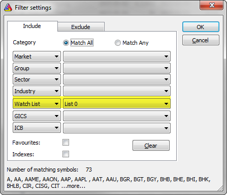
Our test should be applied to a watchlist, which contains all symbols we want to include in our ranking code:

Watch list selection

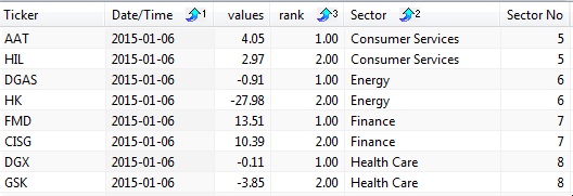
Running the exploration will show two top-ranked symbols for each of the sectors:

Ranking

We can also change Filter variable definition to

Filter 1

and show all ranked symbols instead.

Such ranking information can be used in backtest and sample rules included at the end of the code use rank information to allow only two top-scored symbols to be traded.

Ruin stop or mysterious Short(6) in the trade list

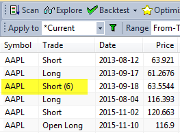
When you back-test a trading system, you may sometimes encounter trades marked with (6) exit reason, showing e.g.: Short (6) or Short (ruin) in the trade list as in the picture below:

Ruin stop in trade list

As explained in the this Knowledge Base article: http://www.amibroker.com/kb/2014/09/24/how-to-identify-which-signal-triggers/ such identifier tells us that the trade was closed because of the ruin stop activation.

A ruin-stop is a built-in, fixed percentage stop set at -99.96%, so it gets activated if your position is losing almost all (99.96%) of its entry value. It almost never occurs in long trades, but it may be quite common if your trading system places short trades without any kind of maximum loss stop. Imagine that you short a stock when its price is $10, then it’s price rises to $20 (twice the entry price). When you buy to cover the position you must pay $20 per share, which means that your loss on this trade is $10 per share ($20-$10). This means 100% loss (as per entry value). If you placed such a trade with all your capital you would be bankrupt. That is why this stop is called “ruin stop”. Unfortunately, by the nature of short selling, the gains are limited to 100% (when stock price goes down to zero) but losses are virtually unlimited.

So what to do to prevent exits by ruin stop?

The best idea is to just place proper max. loss stop at much smaller percentage (such as 10% or 20%) depending on what your risk tolerance is, to limit drawdowns and decrease the chance of wiping your account down to zero.

If, for some weird reason, you want to turn OFF this built-in stop, you can do so using this code:

SetOption"DisableRuinStop"True )

but it is highly discouraged, because when you wipe your account down to zero (or even below zero) it makes no point to run back-test any further. Instead of disabling this feature you should place proper, tighter maximum loss stop.

How does risk-mode trailing stop work?

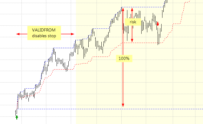
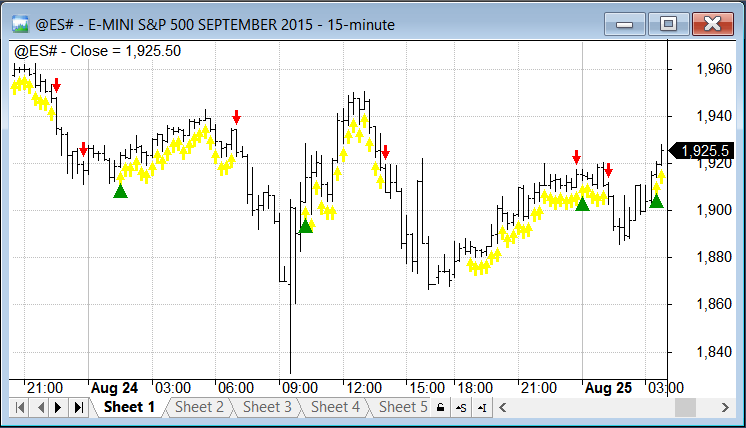
In addition to regular percent or point based stops, AmiBroker allows to define stop size as risk (stopModeRisk), which means that we allow only to give up certain percent of profit gained in given trade. The picture presented below visualizes a risk-mode trailing stop using 35% risk size. Since at the very beginning of the trade profits may be very low (and potentially triggering unwanted exits), this type of stop is best to use with validFrom argument, which allows to delay stop activation by certain number of bars.

The blue line on top represents highest high since entry, while red line shows the stop level calculation, yellow area shows the bars, where our stop has become active:

Risk-mode trailing stop

The above levels were calculated with the following code:

Buy DateNum() == 1140425// custom entry on a fixed date
Sell 0;
BuyPrice SellPrice close;

riskSize 35;
daysDelay 50;

ApplyStopstopTypeTrailingstopModeRiskriskSize1False0daysDelay );
Equity);

priceAtBuy ValueWhenBuyBuyPrice );
highsinceBuy HighestSinceBuyHigh);
stoplevel priceAtBuy + ( highsinceBuy priceAtBuy) * (100-riskSize)/100;

PlotClose"Close"colorDefaultstyleBar );
Plotstoplevel"stop"colorRedstyleDashed );
PlothighsinceBuy"highsinceBuy"colorBluestyleDashed );
PlotpriceAtBuy"priceAtBuy"colorBluestyleDashed );
PlotBarsSinceBuy ) > daysDelay""ColorBlendcolorYellowcolorWhite,0.9), styleArea|styleOwnScale,0,1,0,-1);

PlotShapes(Buy*shapeUpArrowcolorGreen0Low);
PlotShapesIIfSellshapeDownArrowshapeNone), colorRed0High)

Number of stopped-out trades as a custom metric

For the purpose of counting trades closed by particular stop we can refer to ExitReason property of the trade object in the custom backtester. The custom backtest formula presented below iterates through the list of closed trades, then counts the trades, which indicate exit reason = 2, that is stop-loss.

The following values are used for indication of the particular exit reason:

  1. normal exit
  2. maximum loss stop
  3. profit target stop
  4. trailing stop
  5. n-bar stop
  6. ruin stop (losing 99.96% of entry value)
SetCustomBacktestProc"" );

/* Now custom-backtest procedure follows */
if( Status"action" ) == actionPortfolio )
{
    
bo GetBacktesterObject();

    
bo.Backtest(); // run default backtest procedure

    // initialize counter
    
stoplossCountLong stoplossCountShort 0;

    
// iterate through closed trades
    
for( trade bo.GetFirstTrade(); tradetrade bo.GetNextTrade() )
    {

      
// check for stop-loss exit reason
        
if( trade.ExitReason == )
        {
         
// increase long or short counter respectively
            
if( trade.IsLong() )
                
stoplossCountLong++;
            else
                
stoplossCountShort++;
        }
    }

   
// add the custom metric
    
bo.AddCustomMetric"Stoploss trades"stoplossCountLong stoplossCountShort,
                         
stoplossCountLongstoplossCountShort);

}

Buy CrossMACD(), Signal() );
Sell CrossSignal(), MACD() );
Short Sell;
Cover Buy;
ApplyStopstopTypeLossstopModePercent2)

How to run certain piece of code only once

There are situations where we may need to run certain code components just once, e.g. to initialize some static variables before auto-trading execution or perform some tasks (such as ranking) at the very beginning of backtest or exploration. The following techniques may be useful in such cases:

When we want to execute certain part of code just once after starting AmiBroker, we may use a flag written to a static variable that would indicate if our initialization has been triggered or not.

if( NzStaticVarGet("InitializationDone") ) == )
{
   
StaticVarSet("InitializationDone"1);
   
// code for first execution

If we want to run certain part of code at the beginning of the test run in Analysis window, we can use:

if ( Status("stocknum") == )
{
   
// our code here

When Status(“stocknum”) is detected in the code, then execution is performed in a single thread for the very first symbol. Only after processing of this first symbol has finished the other threads will start.

A practical example showing use of this feature is presented in the following tutorial:

http://www.amibroker.com/guide/h_ranking.html

Symbol selection when PositionScore is not defined

AmiBroker’s portfolio backtester allows to define stock ranking and selection criteria by means of PositionScore variable. This is explained in details in the following tutorial chapter:

http://www.amibroker.com/guide/h_portfolio.html

If PositionScore is not defined or it has the same value for two or more symbols, then AmiBroker will use the following rules:

  1. transaction with greater PositionSize is preferred – the comparison method depends on the position sizing approach used in our code:
    • If we use SetPositionSize( dollarvalue, spsValue) – then $ value is compared.
    • If we use SetPositionSize( shares, spsShares) – then number of shares is used for comparison.
    • If we use SetPositionSize( perc, spsPercentOfEquity) – then % equity matters.
  2. alphabetical order
  3. long trades rather than short trades, if both occur at the same time for the same symbol.

How to handle delisted symbols in rotational test

This Knowledge Base article: http://www.amibroker.com/kb/2014/09/26/closing-trades-in-delisted-symbols/ explains how to close trades in delisted symbols in regular backtest (to avoid holding delisted stocks in the trade list and have our max symbol limit impacted by those positions).

In rotational test however we cannot use Sell variable, because trades are driven by symbols’ ranking by PositionScore values. Therefore we would need to assign zero to PositionScore variable for the exit bars respectively – this will force exiting any positions held in given stock.

EnableRotationalTrading();

bi BarIndex();
lastbi LastValuebi ) - Status("BuyDelay");
exitLastBar bi == lastbi;

score /*our regular positionScore*/;
PositionScore IIfexitLastBar 0score )

Note that we are adjusting the last bar index in case trade delays are set in the settings.

As in the regular test, we can also use DelistingDate information if we have it imported into Symbol ->Information window.

EnableRotationalTrading();
exitLastBar datetime() >= GetFnData("DelistingDate");

score /*our regular positionScore*/;
PositionScore IIfexitLastBar 0score )

Limit number of trades per day in a backtest

NOTE: The codes presented below are for intraday data only.

The scenario is as follows: we are intraday traders and we want to limit the number of trades made per day per symbol.

To simulate such scenario in a backtest, we need to count the signals and remove them accordingly after we reach our limit. There are several methods to do so and the choice depends on the signals that our system generates.

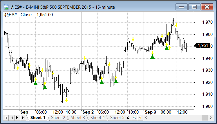
If our trading signals come in a sequence like Buy-Sell-Buy-Sell (without repeated signals in between), then we could just count BUY signals since the beginning of the day and allow first N of these signals, where N is the number of trades we allow. This can be achieved with Sum function:

// trades limit
2;

PlotClose"Close"colorDefaultstyleBar );

// identify new day
dn DateNum();
newDay dn != Refdn,-1);

// buy and sell signals
Buy CrossMACD(), Signal() );
Sell CrossSignal(), MACD() );

// visualize signals with yellow arrows
PlotShapes(Buy*shapeUpArrowcolorYellow0Low);
PlotShapes(Sell*shapeDownArrowcolorYellow0High);

// modify Buy array and allow only first N signals
Buy Buy AND SumBuyBarsSincenewDay) +) <= N;

// visualize modified signals with green triangles
PlotShapes(Buy*shapeUpTrianglecolorGreen0Low, -24)

Price chart

If the signals of the same type may get repeated and occur for example in sequence like Buy-Buy-Buy-Sell, then before counting the entry signals we would first need to remove redundant ones. This can be achieved with Equity( 1 ) function call, which will remove repeated signals the way backtester would handle them:

// trades limit
2;

PlotClose"Close"colorDefaultstyleBar );

// identify new day
dn DateNum();
newDay dn != Refdn, -);

// buy and sell signals
Buy =  MACD() > Signal(); // sample repeated signals
// exit on signal vs macd crossover or last bar of the day
Sell CrossSignal(), MACD() ) OR Refnewday); 

// visualize signals with yellow arrows
PlotShapesBuy*shapeUpArrowcolorYellow0Low );
PlotShapesSell*shapeDownArrowcolorred0High );

// remove redundant signals
Equity);

// modify Buy array and allow only first N signals
Buy Buy AND SumBuyBarsSincenewDay ) + ) <= N;

// visualize modified signals with green triangles
PlotShapesBuy*shapeUpTrianglecolorGreen0Low, -24 )

Price chart

When our trading system uses complex trading rules so we don’t know the order of signals, we can use a loop to process signals and count trades.

// trades limit
2;

PlotClose"Close"colorDefaultstyleBar );

// identify new day
dn DateNum();
newDay dn != Refdn, -);

// buy and sell signals
// sample repeated signals
Buy =  MACD() > Signal();
//exit on signal vs macd crossover or last bar of the day
Sell CrossSignal(), MACD() ) OR Refnewday); 

// visualize signals with yellow arrows
PlotShapesBuy*shapeUpArrowcolorYellow0Low );
PlotShapesSell*shapeDownArrowcolorred0High );

tradeCount onBuy 0;

for( 
0BarCounti++ )
{
    
// reset trade counter on the new day
    
if( newDay] ) tradeCount 0;

    
// keep buy signal if there is no trade and trade count did not hit the limit
    
if( Buy] AND tradeCount AND NOT onBuy )
    {
        
OnBuy 1;
        
TradeCount++;
    }
    else
        
Buy] = 0// ignore other buy signals


if( onBuy AND Sell] )
    {
        
onBuy 0// reset onBuy flag on exit
    
}
}

// visualize modified signals with green triangles
PlotShapesBuy*shapeUpTrianglecolorGreen0Low, -24 )
Next Page »